Creating a class-based TF-IDF with Scikit-Learn
In one of my previous posts, I talked about topic modeling with BERT which involved a class-based version of TF-IDF. This version of TF-IDF allowed me to extract interesting topics from a set of documents.
I thought it might be interesting to go a little bit deeper into the method since it can be used for many more applications than just topic modeling!
An overview of the possible applications:
-
Informative Words per Class: Which words make a class stand-out compared to all others?
-
Class Reduction: Using c-TF-IDF to reduce the number of classes
-
Semi-supervised Modeling: Predicting the class of unseen documents using only cosine similarity and c-TF-IDF
This article will mostly go into the applications of c-TF-IDF but some background on the model will also be given.
If you want to skip all of that and go directly go to the code you can start from the repo here.
Class-based TF-IDF
Before going into the possibilities of this class-based TF-IDF, let us first look at how TF-IDF works and the steps we need to take to transform it into c-TF-IDF.
TF-IDF
TF-IDF is a method for generating features from textual documents which is the result of multiplying two methods:
-
Term Frequency (TF)
-
Inverse Document Frequency (IDF)
The term frequency is simply the raw count of words within a document where each word count is considered a feature.
Inverse document frequency extracts how informative certain words are by calculating a word’s frequency in a document compared to its frequency across all other documents.

You can imagine that words such as the , and , I , etc. are quite common words but contain very little information as they appear in almost every document. Inverse document frequency punishes words that are too common.
The result is a sparse feature matrix that can be used for feature extraction, predictive modeling, and document similarity.
Transform TF-IDF into c-TF-IDF
The goal of the class-based TF-IDF is to supply all documents within a single class with the same class vector. In order to do so, we have to start looking at TF-IDF from a class-based point of view instead of individual documents.
If documents are not individuals, but part of a larger collective, then it might be interesting to actually regard them as such by joining all documents in a class together.
The result would be a very long document that is by itself not actually readable. Imagine reading a document consisting of 10 000 pages!
However, this allows us to start looking at TF-IDF from a class-based perspective.
Then, instead of applying TF-IDF to the newly created long documents, we have to take into account that TF-IDF will take the number of classes instead of the number of documents since we merged documents.
All these changes to TF-IDF results in the following formula:

Where the frequency of each word t is extracted for each class i and divided by the total number of words w. This action can be seen as a form of regularization of frequent words in the class. Next, the total, unjoined, number of documents m is divided by the total frequency of word t across all classes n.
Code
When I introduced c-TF-IDF in the topic modeling with BERT post I used an inefficient method of calculating c-TF-IDF.
Since then, I have created a version of c-TF-IDF that not only allows for a major speed-up but also makes use of the TFidfTransformer in Scikit-Learn which allows us to use the stability that Scikit-Learn has to offer.
import numpy as np
import pandas as pd
import scipy.sparse as sp

from sklearn.preprocessing import normalize
from sklearn.feature_extraction.text import TfidfTransformer, CountVectorizer


class CTFIDFVectorizer(TfidfTransformer):
    def __init__(self, *args, **kwargs):
        super(CTFIDFVectorizer, self).__init__(*args, **kwargs)

    def fit(self, X: sp.csr_matrix, n_samples: int):
        """Learn the idf vector (global term weights) """
        _, n_features = X.shape
        df = np.squeeze(np.asarray(X.sum(axis=0)))
        idf = np.log(n_samples / df)
        self._idf_diag = sp.diags(idf, offsets=0,
                                  shape=(n_features, n_features),
                                  format='csr',
                                  dtype=np.float64)
        return self

    def transform(self, X: sp.csr_matrix) -> sp.csr_matrix:
        """Transform a count-based matrix to c-TF-IDF """
        X = X * self._idf_diag
        X = normalize(X, axis=1, norm='l1', copy=False)
        return X
As you can see, we start from TfidfTransformer and adopt only the fit and transform methods to make it into the CtfidfVectorizer. The vectorizer takes in a sparse matrix that contains the raw count data.
The most basic example to create the c-TF-IDF matrix is as follows:
# Get data
from sklearn.datasets import fetch_20newsgroups
newsgroups = fetch_20newsgroups(subset='train', remove=('headers', 'footers', 'quotes'))

# Create documents per label
docs = pd.DataFrame({'Document': newsgroups.data, 'Class': newsgroups.target})
docs_per_class = docs.groupby(['Class'], as_index=False).agg({'Document': ' '.join})

# Create c-TF-IDF
count = CountVectorizer().fit_transform(docs_per_class.Document)
ctfidf = CTFIDFVectorizer().fit_transform(count, n_samples=len(docs))
We make sure that all documents in class are merged together before passing it through the CountVectorizer to calculate the raw count data which is finally put through the CTFIDFVectorizer.
NOTE: The n_samples passed through the CTFIDFVectorizer is the total number of unjoined documents. This is necessary as the IDF values become too small if the number of joined documents is passed instead.
Applications
As mentioned before, there are roughly three use cases where c-TF-IDF might be interesting to use:
-
Which words are typical for a specific class compared to all others?
-
How can we reduce the number of classes using c-TF-IDF?
-
How can we use c-TF-IDF in predictive modeling?
Informative Words per Class
What makes c-TF-IDF unique compared to TF-IDF is that we can adopt it such that we can search for words that make up certain classes.
If we were to have a class that is marked as space, then we would expect to find space-related words, right?
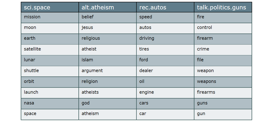
To do this, we simply extract the c-TF-IDF matrix and find the highest values in each class:
# Create bag of words
count_vectorizer = CountVectorizer().fit(docs_per_class.Document)
count = count_vectorizer.transform(docs_per_class.Document)
words = count_vectorizer.get_feature_names()

# Extract top 10 words per class
ctfidf = CTFIDFVectorizer().fit_transform(count, n_samples=len(docs)).toarray()
words_per_class = {newsgroups.target_names[label]: [words[index] for index in ctfidf[label].argsort()[-10:]]
                   for label in docs_per_class.Class}

As expected, the words nicely represent the class they belong to. You can view this c-TF-IDF procedure as a summary of what the class entails.
Class Reduction
At times, having many classes can be detrimental to clear analyses. You might want a more general overview to get a feeling of the major classes in the data.
Fortunately, we can use c-TF-IDF to reduce the number of classes to whatever value you are looking for.
We can do this by comparing the c-TF-IDF vectors of all classes with each other in order to merge the most similar classes:
from sklearn.metrics.pairwise import cosine_similarity

# Get similar classes
distances = cosine_similarity(c_tf_idf, c_tf_idf)
np.fill_diagonal(distances, 0)

# For each class, extract the most similar class
result = pd.DataFrame([(newsgroups.target_names[index],
                        newsgroups.target_names[distances[index].argmax()])
                       for index in range(len(docs_per_class))],
                      columns=["From", "To"])

Using the cosine similarity on the c-TF-IDF vectors seems to have worked! We correctly find that the classes atheism and christian can be merged in what we can call religion. We find similar results for autos and motorcycles which can be combined together.
Using this method, we can select the most similar classes and combine them as long as they are similar enough.
Semi-supervised Modeling
Using c-TF-IDF we can even perform semi-supervised modeling directly without the need for a predictive model.
We start by creating a c-TF-IDF matrix for the train data. The result is a vector per class which should represent the content of that class. Finally, we check, for previously unseen data, how similar that vector is to that of all categories:
from sklearn import metrics
from sklearn.datasets import fetch_20newsgroups
from sklearn.metrics.pairwise import cosine_similarity

# Get train data
train = fetch_20newsgroups(subset='train', remove=('headers', 'footers', 'quotes'))
docs = pd.DataFrame({'Document': train.data, 'Class': train.target})
docs_per_class = docs.groupby(['Class'], as_index=False).agg({'Document': ' '.join})

# Create c-TF-IDF based on the train data
count_vectorizer = CountVectorizer().fit(docs_per_class.Document)
count = count_vectorizer.transform(docs_per_class.Document)
ctfidf_vectorizer = CTFIDFVectorizer().fit(count, n_samples=len(docs))
ctfidf = ctfidf_vectorizer.transform(count)

# Predict test data
test = fetch_20newsgroups(subset='test', remove=('headers', 'footers', 'quotes'))
count = count_vectorizer.transform(test.data)
vector = ctfidf_vectorizer.transform(count)
distances = cosine_similarity(vector, ctfidf)
prediction = np.argmax(distances, 1)

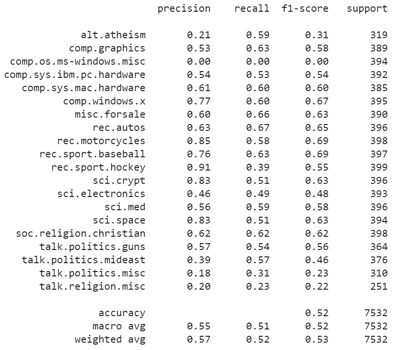
print(metrics.classification_report(test.target, prediction, target_names=test.target_names))

Although we can see that the results are nothing to write home about with an accuracy of roughly 50%… The accuracy is much better than randomly guessing the class which is 5%.
Without any complex predictive model, we managed to get decent accuracy with a fast and relatively simple model. We did not even preprocess the data!
Thank you for reading!
If you are, like me, passionate about AI, Data Science, or Psychology, please feel free to add me on LinkedIn or follow me on Twitter.
All examples and code in this article can be found here.