Tips for Advanced Feature Engineering

Arguably, two of the most important steps in developing a machine learning model is feature engineering and preprocessing. Feature engineering consists of the creation of features whereas preprocessing involves cleaning the data.

Torture the data, and it will confess to anything. — Ronald Coase

We often spend a significant amount of time refining the data into something useful for modeling purposes. In order to make this work more efficient, I would like to share 4 Tips and Tricks that could help you with engineering and preprocessing those features.

I should note that, how cliche it might be, domain knowledge might be one of the most important things to have when engineering features. It might help you in preventing under- and overfitting by having a better understanding of the features that you use.

You can find the notebook with analyses here.

1. Resampling Imbalanced Data

In practice, you will encounter imbalanced data more often than not. This does not necessarily have to be a problem if your target only has a slight imbalance. You could then resolve it by using proper validation measures for the data such as Balanced Accuracy, Precision-Recall Curves or F1-score.

Unfortunately, this is not always the case and your target variable might be highly imbalanced (e.g., 10:1). Instead, you can oversample the minority target in order to introduce balance using a technique called SMOTE.

SMOTE

SMOTE stands for Synthetic Minority Oversampling Technique and is an oversampling technique used to increase the samples in a minority class.

It generates new samples by looking at the feature space of the target and detecting nearest neighbors. Then, it simply selects similar samples and changes a column at a time randomly within the feature space of the neighboring samples.

The module to implement SMOTE can be found within the imbalanced-learn package. You can simply import the package and apply a fit_transform:

import pandas as pd
from imblearn.over_sampling import SMOTE

# Import data and create X, y
df = pd.read_csv('creditcard_small.csv')
X = df.iloc[:,:-1]
y = df.iloc[:,-1].map({1:'Fraud', 0:'No Fraud'})

# Resample data
X_resampled, y_resampled = SMOTE(sampling_strategy={"Fraud":1000}).fit_resample(X, y)
X_resampled = pd.DataFrame(X_resampled, columns=X.columns)

Original data (LEFT) versus oversampled data (RIGHT).

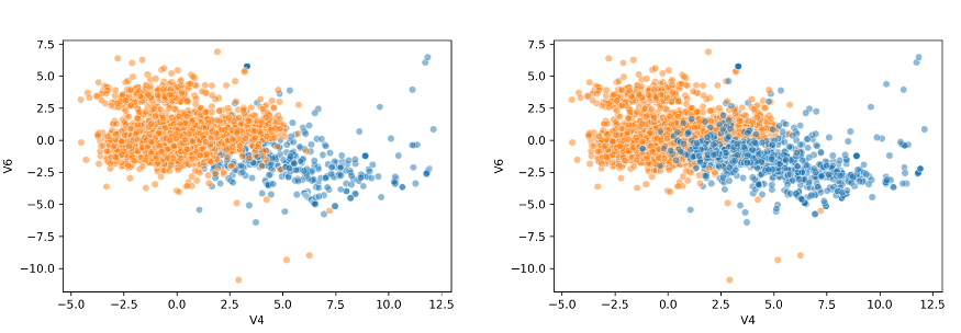
As you can see the model successfully oversampled the target variable. There are several strategies that you can take when oversampling using SMOTE: * 'minority': resample only the minority class; * 'not minority': resample all classes but the minority class; * 'not majority': resample all classes but the majority class; * 'all': resample all classes; * When dict, the keys correspond to the targeted classes. The values correspond to the desired number of samples for each targeted class.

I chose to use a dictionary to specify the extent to which I wanted to oversample my data.

Additional tip 1: If you have categorical variables in your dataset SMOTE is likely to create values for those variables that cannot happen. For example, if you have a variable called isMale, which could only take 0 or 1, then SMOTE might create 0.365 as a value.

Instead, you can use SMOTENC which takes into account the nature of categorical variables. This version is also available in the imbalanced-learn package.

Additional tip 2: Make sure to oversample after creating the train/test split so that you only oversample the train data. You typically do not want to test your model on synthetic data.

2. Creating New Features

To improve the quality and predictive power of our models, new features from existing variables are often created. We can create some interaction (e.g., multiply or divide) between each pair of variables hoping to find an interesting new feature. This, however, is a lengthy process and requires a significant amount of coding. Fortunately, this can be automated using Deep Feature Synthesis.

Deep Feature Synthesis

Deep feature synthesis (DFS) is an algorithm which enables you to quickly create new variables with varying depth. For example, you can multiply pairs of columns but you can also choose to first multiply Column A with Column B and then add Column C.

First, let me introduce the data I will be using for the example. I have chosen to use HR analytics data since the features are easily interpretable:

Simply based on our intuition we could identify average_monthly_hours divided by number_project as an interesting new variable. However, there might be much more relationships that we miss out on if we only follow intuition.

The package does require an understanding of their use of Entities. However, if you use a single table you can simply follow the code below:

import featuretools as ft
import pandas as pd

# Create Entity
turnover_df = pd.read_csv('turnover.csv')
es = ft.EntitySet(id = 'Turnover')
es.entity_from_dataframe(entity_id = 'hr', dataframe = turnover_df, index = 'index')

# Run deep feature synthesis with transformation primitives
feature_matrix, feature_defs = ft.dfs(entityset = es, target_entity = 'hr',
                                      trans_primitives = ['add_numeric', 'multiply_numeric'], 
                                      verbose=True)

The first step is to create an entity from which relationships can be created with other tables if necessary. Next, we can simply run ft.dfs in order to create new variables. We specify how variables are created with the parameter trans_primitives. We chose to either add numeric variables together or multiply.

As you can see in the image above we have created an additional 668 features using only a few lines of code. A few examples of the features that were created: * last_evaluation multiplied with satisfaction_level * left multiplied with promotion_last_5years * average_monthly_hours multiplied with satisfaction_level plus time_spend_company

Additional tip 1: Note that the implementation here is relatively basic. The great thing about DFS is that it can create new variables from aggregations between tables (e.g., facts and dimensions). See this link for an example.

Additional tip 2: Run ft.list_primitives()in order to see the full list of aggregation that you can do. It even handles timestamps, null values, and long/lat information.

3. Handling Missing Values

As always, there is no one best way of dealing with missing values. Depending on your data it might be sufficient to simply fill them with the mean or mode of certain groups. However, there are advanced techniques that use known parts of the data to impute the missing values.

One such method is called IterativeImputer a new package in Scikit-Learn which is based on the popular R algorithm for imputing missing variables, MICE.

Iterative Imputer

Although python is a great language for developing machine learning models, there are still quite a few methods that work better in R. An example is the well-establish imputation packages in R: missForest, mi, mice, etc.

The Iterative Imputer is developed by Scikit-Learn and models each feature with missing values as a function of other features. It uses that as an estimate for imputation. At each step, a feature is selected as output y and all other features are treated as inputs X. A regressor is then fitted on X and y and used to predict the missing values of y. This is done for each feature and repeated for several imputation rounds.

Let us take a look at an example. The data that I use is the well known Titanic dataset. In this dataset, the column Age has missing values that we would like to fill. The code, as always, is straightforward:

# explicitly require this experimental feature
# now you can import normally from sklearn.impute
from sklearn.experimental import enable_iterative_imputer  
from sklearn.impute import IterativeImputer

from sklearn.ensemble import RandomForestRegressor
import pandas as pd

# Load data
titanic = pd.read_csv("titanic.csv")
titanic = titanic.loc[:, ['Pclass', 'Age', 'SibSp', 'Parch', 'Fare']]

# Run imputer with a Random Forest estimator
imp = IterativeImputer(RandomForestRegressor(), max_iter=10, random_state=0)
titanic = pd.DataFrame(imp.fit_transform(titanic), columns=titanic.columns)

The great thing about this method is that it allows you to use an estimator of your choosing. I used a RandomForestRegressor to mimic the behavior of the frequently used missForest in R.

Additional tip 1: If you have sufficient data, then it might be an attractive option to simply delete samples with missing data. However, keep in mind that it could create bias in your data. Perhaps the missing data follows a pattern that you miss out on.

Additional tip 2: The Iterative Imputer allows for different estimators to be used. After some testing, I found out that you can even use Catboost as an estimator! Unfortunately, LightGBM and XGBoost do not work since their random state names differ.

4. Outlier Detection

Outliers are difficult to detect without a good understanding of the data. If you know the data well you can more easily specify the thresholds at which your data still makes sense.

At times this is not possible since a perfect understanding of the data is difficult to achieve. Instead, you can make use of Outlier Detection algorithms such as the popular Isolation Forest.

Isolation Forest

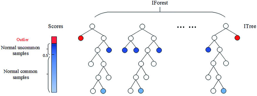
In the Isolation Forest Algorithm, the keyword is Isolation. In essence, the algorithm checks how easily a sample can be isolated. This results in an isolation number which is calculated by the number of splits, in a Random Decision Tree, needed to isolate a sample. This isolation number is then averaged over all trees.

If the algorithm only needs to do a few splits to find a sample, then it is more likely to be an outlier. The splits themselves are also randomly partitioned such that it produces shorter paths for anomalies. Thus, when the isolation number across all trees is low, then that sample is highly likely to be an anomaly.

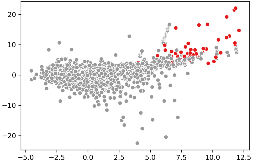
To show an example I again used the credit card dataset that we used before:

from sklearn.ensemble import IsolationForest
import pandas as pd
import seaborn as sns

# Predict and visualize outliers
credit_card = pd.read_csv('creditcard_small.csv').drop("Class", 1)
clf = IsolationForest(contamination=0.01, behaviour='new')
outliers = clf.fit_predict(credit_card)
sns.scatterplot(credit_card.V4, credit_card.V2, outliers, palette='Set1', legend=False)

Additional Tip 1: There is an extended version of the Isolation Forest available that improves on some shortcomings. However, there have been mixed reviews.