Validating your Machine Learning Model
I believe that one of the most underrated aspects of creating your Machine Learning Model is thorough validation. Using proper validation techniques helps you understand your model, but most importantly, estimate an unbiased generalization performance.
There is no single validation method that works in all scenarios. It is important to understand if you are dealing with groups, time-indexed data, or if you are leaking data in your validation procedure.
Which validation method is right for my use case?
When researching these aspects I found plenty of articles describing evaluation techniques, but validation techniques typically stop at k-Fold cross-validation.
I would like to show you the world that uses k-Fold CV and goes one step further into Nested CV, LOOCV, but also into model selection techniques.
The following methods for validation will be demonstrated:
- Train/test split
- k-Fold Cross-Validation
- Leave-one-out Cross-Validation
- Leave-one-group-out Cross-Validation
- Nested Cross-Validation
- Time-series Cross-Validation
- Wilcoxon signed-rank test
- McNemar’s test
- 5x2CV paired t-test
- 5x2CV combined F test
1. Splitting your data
The basis of all validation techniques is splitting your data when training your model. The reason for doing so is to understand what would happen if your model is faced with data it has not seen before.
Train/test split
The most basic method is the train/test split. The principle is simple, you simply split your data randomly into roughly 70% used for training the model and 30% for testing the model.
# Creating a train/test split with X being your features and y the target
import numpy as np
from sklearn.model_selection import train_test_split
X, y = np.arange(10).reshape((5, 2)), range(5)
(X_train, X_test,
 y_train, y_test) = train_test_split(X, y, test_size=0.3,
                                     random_state=42)
The benefit of this approach is that we can see how the model reacts to previously unseen data.
However, what if one subset of our data only have people of a certain age or income levels? This is typically referred to as a sampling bias:
Sampling bias is systematic error due to a non-random sample of a population, causing some members of the population to be less likely to be included than others, resulting in a biased sample.

Before going into methods that help with the sampling bias (like k-Fold cross-validation), I would like to go into the additional holdout set.
Holdout set
When optimizing the hyperparameters of your model, you might overfit your model if you were to optimize using the train/test split.
Why? Because the model searches for the hyperparameters that fit the specific train/test you made.
To solve this issue, you can create an additional holdout set. This is often 10% of the data which you have not used in any of your processing/validation steps.

After optimizing your model on the train/test split, you can check if you did not overfit by validating on your holdout set.
TIP: If only use a train/test split, then I would advise comparing the distributions of your train and test sets. If they differ significantly, then you might run into problems with generalization. Use Facets to easily compare their distributions.
2. k-Fold Cross-Validation (k-Fold CV)
To minimize sampling bias we can think about approach validation slightly different. What if, instead of making a single split, we make many splits and validate on all combinations of those splits?
This is where k-fold cross-validation comes in. It splits the data into k folds, then trains the data on k-1 folds and test on the one fold that was left out. It does this for all combinations and averages the result on each instance.
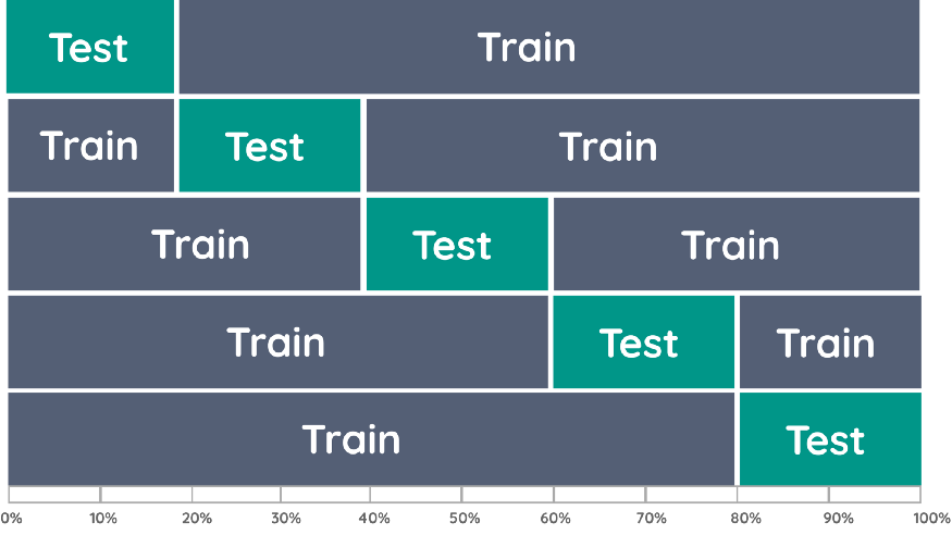
The advantage is that all observations are used for both training and validation, and each observation is used once for validation. We typically choose either i=5 or k=10 as they find a nice balance between computational complexity and validation accuracy:
import numpy as np
from sklearn.model_selection import KFold
X = np.array([[1, 2], [3, 4], [1, 2], [3, 4]])
y = np.array([1, 2, 3, 4])
kf = KFold(n_splits=5)

for train_index, test_index in kf.split(X):
    X_train, X_test = X[train_index], X[test_index]
    y_train, y_test = y[train_index], y[test_index]
TIP: The scores of each fold from cross-validation techniques are more insightful than one may think. They are mostly used to simply extract the average performance. However, one might also look at the variance or standard deviation of the resulting folds as it will give information about the stability of the model across different data inputs.
3. Leave-one-out Cross-Validation (LOOCV)
A variant of k-Fold CV is Leave-one-out Cross-Validation (LOOCV). LOOCV uses each sample in the data as a separate test set while all remaining samples form the training set. This variant is identical to k-fold CV when k = n (number of observations).
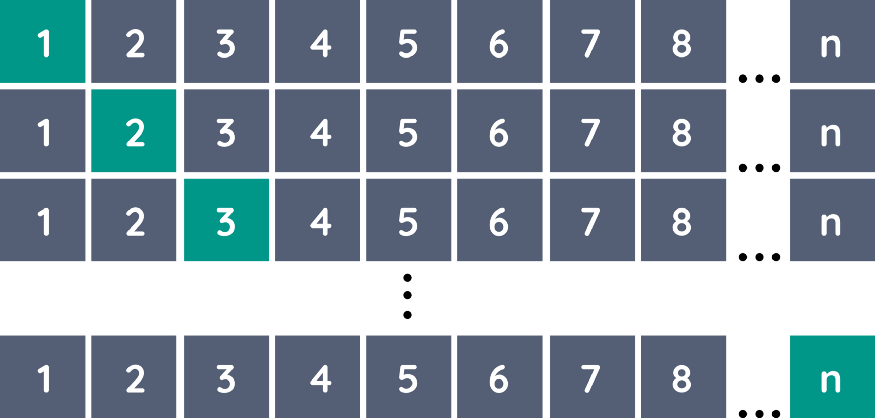
It can be easily implemented using sklearn:
import numpy as np
from sklearn.model_selection import LeaveOneOut
X = np.array([[1, 2], [3, 4]])
y = np.array([1, 2])
loo = LeaveOneOut()

for train_index, test_index in loo.split(X):
  X_train, X_test = X[train_index], X[test_index]
  y_train, y_test = y[train_index], y[test_index]
NOTE: LOOCV is computationally very costly as the model needs to be trained n times. Only do this if the data is small or if you can handle that many computations.
Leave-one-group-out Cross-Validation (LOGOCV)
The issue with k-Fold CV is that you might want each fold to only contain a single group. For example, let’s say you have a dataset of 20 companies and their clients and you want to predict the success of these companies.
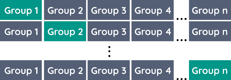
To keep the folds “pure” and only contain a single company you would create a fold for each company. That way, you create a version of k-Fold CV and LOOCV where you leave one company/group out.
Again, implementation can be done using sklearn:
import numpy as np
from sklearn.model_selection import LeaveOneGroupOut
X = np.array([[1, 2], [3, 4], [5, 6], [7, 8]])
y = np.array([1, 2, 1, 2])
groups = np.array([1, 1, 2, 2])

logo = LeaveOneGroupOut()

for train_index, test_index in logo.split(X, y, groups):
    X_train, X_test = X[train_index], X[test_index]
    y_train, y_test = y[train_index], y[test_index]
4. Nested Cross-Validation
When you are optimizing the hyperparameters of your model and you use the same k-Fold CV strategy to tune the model and evaluate performance you run the risk of overfitting. You do not want to estimate the accuracy of your model on the same split that you found the best hyperparameters for.
Instead, we use a Nested Cross-Validation strategy allowing to separate the hyperparameter tuning step from the error estimation step. To do this, we nest two k-fold cross-validation loops: * The inner loop for hyperparameter tuning and * the outer loop for estimating accuracy.
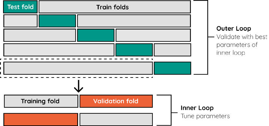
The example below shows an implementation using k-Fold CV for both the inner and outer loop.
from sklearn.datasets import load_iris
from sklearn.svm import SVC
from sklearn.model_selection import GridSearchCV, cross_val_score, KFold

# Load the dataset
X_iris = load_iris().data
y_iris = load_iris().target

# Set up possible values of parameters to optimize over
p_grid = {"C": [1, 10, 100],
          "gamma": [.01, .1]}

# We will use a Support Vector Classifier with "rbf" kernel
svr = SVC(kernel="rbf")

# Create inner and outer strategies
inner_cv = KFold(n_splits=2, shuffle=True, random_state=42)
outer_cv = KFold(n_splits=5, shuffle=True, random_state=42)

# Pass the gridSearch estimator to cross_val_score
clf = GridSearchCV(estimator=svr, param_grid=p_grid, cv=inner_cv)
nested_score = cross_val_score(clf, X=X_iris, y=y_iris, cv=outer_cv).mean(); print(nested_score)
You are free to select the cross-validation approaches you use in the inner and outer loops. For example, you can use Leave-one-group-out for both the inner and outer loops if you want to split by specific groups.
5. Time Series CV
Now, what would happen if you were to use k-Fold CV on time series data? Overfitting would be a major concern since your training data could contain information from the future. It is important that all your training data happens before your test data.
One way of validating time series data is by using k-fold CV and making sure that in each fold the training data takes place before the test data.

Fortunately, sklearn is again to the rescue and has a Time Series CV builtin:
import numpy as np
from sklearn.model_selection import TimeSeriesSplit
X = np.array([[1, 2], [3, 4], [1, 2], [3, 4], [1, 2], [3, 4]])
y = np.array([1, 2, 3, 4, 5, 6])
tscv = TimeSeriesSplit(n_splits=5)

for train_index, test_index in tscv.split(X):
    X_train, X_test = X[train_index], X[test_index]
    y_train, y_test = y[train_index], y[test_index]
NOTE: Make sure to order your data according to the time index that you use seeing as you do not supply the TimeSeriesSplit with a time index. Thus, it will create the split simply based on the order in which the records appear.
6. Comparing Models
When do you consider one model to be better than another? If one model’s accuracy is insignificantly higher than another, is that a sufficient enough reason for choosing the best model?
As a Data Scientist, I want to make sure that I understand if a model is actually significantly more accurate than another. Fortunately, many methods exist that apply statistics to the selection of Machine Learning models.
Wilcoxon signed-rank test
One such method is the Wilcoxon signed-rank test which is the non-parametric version of the paired Student’s t-test. It can be used when the sample size is small and the data does not follow a normal distribution.
We can apply this significance test for comparing two Machine Learning models. Using k-fold cross-validation we can create, for each model, k accuracy scores. This will result in two samples, one for each model.
Then, we can use the Wilcoxon signed-rank test to test if the two samples differ significantly from each other. If they do, then one is more accurate than the other.

Below, you can see an implementation of this procedure.
from scipy.stats import wilcoxon
from sklearn.datasets import load_iris
from sklearn.ensemble import ExtraTreesClassifier, RandomForestClassifier
from sklearn.model_selection import cross_val_score, KFold

# Load the dataset
X = load_iris().data
y = load_iris().target

# Prepare models and select your CV method
model1 = ExtraTreesClassifier()
model2 = RandomForestClassifier()
kf = KFold(n_splits=20, random_state=42)

# Extract results for each model on the same folds
results_model1 = cross_val_score(model1, X, y, cv=kf)
results_model2 = cross_val_score(model2, X, y, cv=kf)

# Calculate p value
stat, p = wilcoxon(results_model1, results_model2, zero_method='zsplit'); p
The result will be a p-value. If that value is lower than 0.05 we can reject the null hypothesis that there are no significant differences between the models.
NOTE: It is important that you keep the same folds between the models to make sure the samples are drawn from the same population. This is achieved by simply setting the same random_state in the cross-validation procedure.
McNemar’s Test
McNemar’s test is used to check the extent to which the predictions between one model and another match. This is referred to as the homogeneity of the contingency table. From that table, we can calculate x² which can be used to compute the p-value:

Again, if the p-value is lower than 0.05 we can reject the null hypothesis and see that one model is significantly better than the other.
We can use mlxtend package to create the table and calculate the corresponding p-value:
import numpy as np
from mlxtend.evaluate import mcnemar_table, mcnemar

# The correct target (class) labels
y_target = np.array([0, 0, 0, 0, 0, 0, 0, 0, 0, 0, 0,
                     1, 1, 1, 1, 1, 1, 1, 1, 1, 1, 1])

# Class labels predicted by model 1
y_model1 = np.array([0, 1, 0, 0, 0, 1, 1, 0, 0, 0, 0,
                     0, 1, 1, 0, 0, 1, 1, 0, 1, 1, 1])

# Class labels predicted by model 2
y_model2 = np.array([0, 0, 1, 1, 0, 1, 0, 0, 0, 0, 0,
                     1, 1, 0, 0, 0, 1, 1, 0, 0, 0, 0])

# Calculate p value
tb = mcnemar_table(y_target=y_target,
                   y_model1=y_model1,
                   y_model2=y_model2)
chi2, p = mcnemar(ary=tb, exact=True)

print('chi-squared:', chi2)
print('p-value:', p)
5x2CV paired t-test
The 5x2CV paired t-test is a method often used to compare Machine Learning models due to its strong statistical foundation.
The method works as follows. Let’s say we have two classifiers, A and B. We randomly split the data in 50% training and 50% test. Then, we train each model on the training data and compute the difference in accuracy between the models from the test set, called DiffA. Then, the training and test splits are reversed and the difference is calculated again in DiffB.
This is repeated five times after which the mean variance of the differences is computed (S²). Then, it is used to calculate the t-statistic:

Where DiffA₁ is the mean variance of the first iteration.

Again, we can use the mlxtend package to calculate the corresponding p-value:
from mlxtend.evaluate import paired_ttest_5x2cv
from sklearn.tree import DecisionTreeClassifier, ExtraTreeClassifier
from mlxtend.data import iris_data

# Prepare data and clfs
X, y = iris_data()
clf1 = ExtraTreeClassifier()
clf2 = DecisionTreeClassifier()

# Calculate p-value
t, p = paired_ttest_5x2cv(estimator1=clf1,
                          estimator2=clf2,
                          X=X, y=y,
                          random_seed=1)
NOTE: You can use the combined 5x2CV F-test instead which was shown to be slightly more robust (Alpaydin, 1999). This method is implemented in mlxtend as from mlxtend.evaluate import combined_ftest_5x2cv.
Conclusion
Validation can be a tricky subject as it requires significant understanding of the data in order to select the correct procedure. Hopefully, this helped you get some feeling of the methods that are often used for validation.
All code can be found here.